Introduction
In 1992, New Jersey raised its minimum wage while neighboring Pennsylvania did not. David Card and Alan Krueger exploited this policy discontinuity as a natural experiment: fast-food restaurants in eastern Pennsylvania serve as a comparison group for restaurants in New Jersey that faced the same local demand shocks but not the same minimum-wage shock. The authors surveyed stores before and after the policy change and compared employment, wages, and prices across states and across waves.
The paper became famous because it challenged a simple textbook prediction that a higher minimum wage must reduce employment, at least in the short run, in a low-wage, high-turnover industry where firms have some wage-setting power and adjustment margins beyond immediate layoffs. The “NJ vs. PA” comparison is the key identification move: it supplies a plausible counterfactual trend for what would have happened in New Jersey absent the reform.
This post replicates the headline tables from the paper (Table 2, the upper-left (3) block of Table 3, and Table 4 column (i)) using the public-use flat file (public.dat), the ASCII codebook, and the variable logic in David Card’s check.sas replication file.
For reproducibility, I also embed screenshots of the published tables alongside my reproduced numbers.
Methodological note: why DiD is stronger than “NJ only”
A before-and-after comparison in New Jersey alone conflates the minimum wage increase with any aggregate trend affecting fast-food employment between early 1992 and late 1992 (seasonality, local demand, macro shocks, supply disruptions, and so on). A Pennsylvania control group is meant to absorb those common shocks under a parallel trends assumption: absent the policy, NJ and PA would have evolved similarly. The difference-in-differences estimand compares changes across states, which removes time-invariant differences between regions and isolates a policy-induced shift relative to a credible counterfactual trend.
Data processing
The public-use file is fixed-width ASCII (410 stores). Column locations follow the codebook file in njmin/, and variable definitions follow check.sas (for example, EMPTOT and GAP).
Table 2 (published means + standard errors)
Card and Krueger’s Table 2 summarizes store composition and Wave 1 / Wave 2 means for a set of key variables. Below, I reproduce the same rows shown in your screenshot (store-type shares, FTE, % full-time, wages, meal price, hours, recruiting bonus).
Standard errors are computed as (s / ) within each state, where (s) is the sample standard deviation and (n) is the count of non-missing stores for that variable.
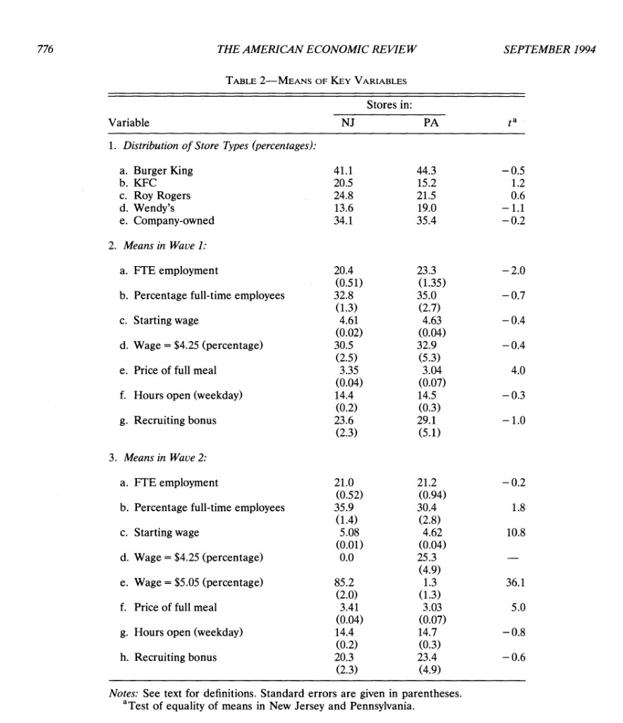
Table 3 (the (3) block: columns (i)–(iii), rows 1–3)
This is the “NJ vs PA” comparison in the top-left of Table 3:
- Columns: Pennsylvania, New Jersey, NJ − PA
- Rows: Wave 1 mean FTE, Wave 2 mean FTE, change in mean FTE (mean after − mean before)
Closures: following the paper’s discussion, permanently closed stores (STATUS2 = 3) have Wave 2 employment set to 0 when computing Wave 2 means. (Temporarily closed / missing Wave 2 employment are handled as missing in these first rows, matching the published counts like (n=319) for NJ Wave 2 FTE.)
Rows 1–2: standard errors are (s/) within each state, as in Table 2.
Row 3 (change): the point estimate is mean(Wave 2 FTE) − mean(Wave 1 FTE) in each state (the same object CK prints in the table). The standard errors in parentheses for PA and NJ are (s_{}/) where (_i =) Wave 2 − Wave 1 for stores with non-missing FTE in both waves (a paired cohort). That rule matches CK’s Pennsylvania (1.25) very closely on this public file; New Jersey is a bit below CK’s (0.54), which is expected when Wave‑1 and Wave‑2 samples differ slightly in the ASCII extract.
For NJ − PA, the standard error is () using the row‑3 state standard errors above.
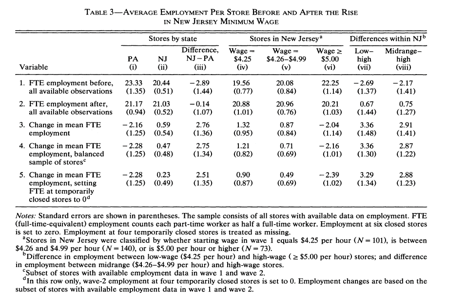
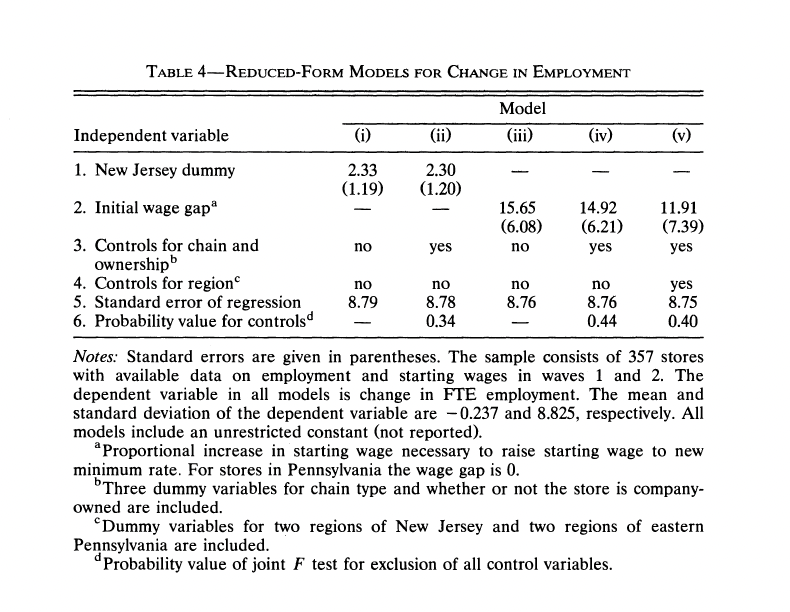
Table 4, column (i): OLS of ΔFTE on the NJ dummy
This is the simplest “difference-in-differences in regression form” specification:
ΔFTEi = α + β ⋅ NJi + ui
To match the paper’s Table 4 footnote (“357 stores with available data in both waves”), I use the C1 subset logic from check.sas:
DEMP(here: (FTE)) is non-missing, and- either the store is permanently closed in Wave 2 (
STATUS2 = 3), or the store has a non-missing wage change (wage = wage_{2}-wage_{1}).
This is exactly the IF CLOSED=1 OR (CLOSED=0 AND DWAGE NE .); filter in check.sas, and it yields (n=357) in this ASCII public-use file.
Standard errors are the homoskedastic OLS standard errors (not HC1), matching the style of the published table.
Card and Krueger’s printed Table 4 does not list the intercept, (t)-statistics, or (p)-values for column (i); it reports the NJ dummy (coefficient with SE in parentheses), no chain/region controls, and the standard error of the regression (RMSE). The replication below uses that same layout; the intercept is still estimated in the OLS (it equals the mean ()FTE in Pennsylvania in this sample) but is omitted from the table to match the paper.
Visual Summary: Difference-in-Differences
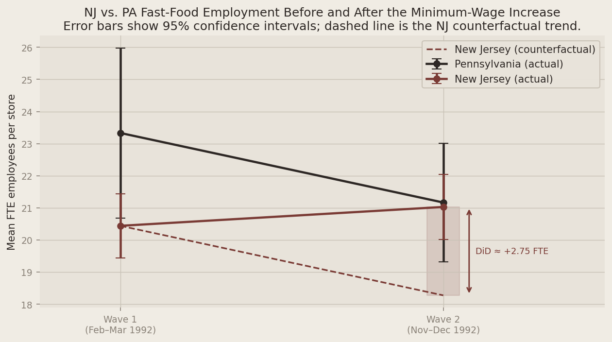
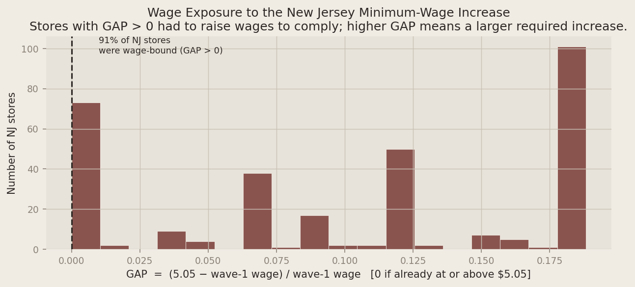
The plots below make the Table 3 numbers concrete. The first shows the parallel-trends logic: Pennsylvania’s trend is the counterfactual for what would have happened in New Jersey absent the reform. The dashed line extends New Jersey’s Wave-1 level by the same amount Pennsylvania changed — any gap between that line and New Jersey’s actual Wave-2 outcome is the DiD estimate. The second plot shows the distribution of the wage gap (GAP) among New Jersey stores, which captures how exposed each store was to the new minimum.
Show Python code
from __future__ import annotations

from pathlib import Path

import matplotlib.pyplot as plt
import numpy as np
import pandas as pd
import seaborn as sns
import statsmodels.api as sm
from IPython.display import Markdown, display


def markdown_table(headers: list[str], rows: list[list[str]]) -> str:
    out = []
    out.append("| " + " | ".join(headers) + " |")
    out.append("| " + " | ".join(["---"] * len(headers)) + " |")
    for r in rows:
        out.append("| " + " | ".join(r) + " |")
    return "\n".join(out)


plt.rcParams.update({
    "figure.facecolor": "#f0ece4",
    "axes.facecolor":   "#e8e3da",
    "axes.grid": True,
    "grid.color": "#c9c2b6",
    "grid.linewidth": 0.7,
    "axes.spines.top": False,
    "axes.spines.right": False,
    "axes.spines.left": False,
    "axes.spines.bottom": False,
    "font.family": "sans-serif",
    "axes.titlesize": 12,
    "axes.labelsize": 10,
    "xtick.labelsize": 9,
    "ytick.labelsize": 9,
    "text.color": "#2e2825",
    "axes.labelcolor": "#2e2825",
    "xtick.color": "#8a8278",
    "ytick.color": "#8a8278",
})

DATA_PATH = Path("njmin/public.dat")

# Codebook columns are 1-based inclusive; pandas colspecs are 0-based [start, end).
colspecs = [
    ("SHEET", 0, 3),
    ("CHAIN", 4, 5),
    ("CO_OWNED", 6, 7),
    ("STATE", 8, 9),
    ("SOUTHJ", 10, 11),
    ("CENTRALJ", 12, 13),
    ("NORTHJ", 14, 15),
    ("PA1", 16, 17),
    ("PA2", 18, 19),
    ("SHORE", 20, 21),
    ("NCALLS", 22, 24),
    ("EMPFT", 25, 30),
    ("EMPPT", 31, 36),
    ("NMGRS", 37, 42),
    ("WAGE_ST", 43, 48),
    ("INCTIME", 49, 54),
    ("FIRSTINC", 55, 60),
    ("BONUS", 61, 62),
    ("PCTAFF", 63, 68),
    ("MEALS", 69, 70),
    ("OPEN", 71, 76),
    ("HRSOPEN", 77, 82),
    ("PSODA", 83, 88),
    ("PFRY", 89, 94),
    ("PENTREE", 95, 100),
    ("NREGS", 101, 103),
    ("NREGS11", 104, 106),
    ("TYPE2", 107, 108),
    ("STATUS2", 109, 110),
    ("DATE2", 111, 117),
    ("NCALLS2", 118, 120),
    ("EMPFT2", 121, 126),
    ("EMPPT2", 127, 132),
    ("NMGRS2", 133, 138),
    ("WAGE_ST2", 139, 144),
    ("INCTIME2", 145, 150),
    ("FIRSTIN2", 151, 156),
    ("SPECIAL2", 157, 158),
    ("MEALS2", 159, 160),
    ("OPEN2R", 161, 166),
    ("HRSOPEN2", 167, 172),
    ("PSODA2", 173, 178),
    ("PFRY2", 179, 184),
    ("PENTREE2", 185, 190),
    ("NREGS2", 191, 193),
    ("NREGS112", 194, 196),
]

df = pd.read_fwf(
    DATA_PATH,
    colspecs=[(a, b) for _, a, b in colspecs],
    names=[n for n, _, _ in colspecs],
    dtype=str,
)

for c in df.columns:
    df[c] = df[c].str.strip()

num_cols = [c for c in df.columns if c != "SHEET"]
df[num_cols] = df[num_cols].apply(pd.to_numeric, errors="coerce")

df["NJ"] = (df["STATE"] == 1).astype(int)

df["FTE_W1"] = df["EMPFT"] + df["NMGRS"] + 0.5 * df["EMPPT"]
df["FTE_W2_RAW"] = df["EMPFT2"] + df["NMGRS2"] + 0.5 * df["EMPPT2"]

# Permanently closed stores get Wave-2 FTE set to 0, per Card & Krueger's methodology.
df["FTE_W2"] = np.where(df["STATUS2"] == 3, 0.0, df["FTE_W2_RAW"])

df["PMEAL_W1"] = df["PSODA"] + df["PFRY"] + df["PENTREE"]
df["PMEAL_W2"] = df["PSODA2"] + df["PFRY2"] + df["PENTREE2"]

# % full-time employees (CK definition used in replications: EMPFT / EMPTOT, where EMPTOT = FTE)
df["PFT_W1"] = np.where(df["FTE_W1"] > 0, df["EMPFT"] / df["FTE_W1"], np.nan)
df["PFT_W2"] = np.where(df["FTE_W2"] > 0, df["EMPFT2"] / df["FTE_W2"], np.nan)

# Wage indicators
df["WAGE425_W1"] = (df["WAGE_ST"] == 4.25).astype(float)
df["WAGE425_W2"] = (df["WAGE_ST2"] == 4.25).astype(float)
df["WAGE505_W2"] = (df["WAGE_ST2"] == 5.05).astype(float)

# Recruiting bonus indicators (0/1 in public data)
df["BONUS_W1"] = (df["BONUS"] == 1).astype(float)
df["BONUS_W2"] = (df["SPECIAL2"] == 1).astype(float)

# Wage change (used for Table 4 sample selection in check.sas)
df["DWAGE"] = df["WAGE_ST2"] - df["WAGE_ST"]

# GAP definition from check.sas (useful for extensions beyond Table 4 col. (i))
df["GAP"] = np.where(df["STATE"] == 0, 0.0, np.nan)
mask_nj_below = (df["STATE"] == 1) & df["WAGE_ST"].notna()
df.loc[mask_nj_below & (df["WAGE_ST"] >= 5.05), "GAP"] = 0.0
df.loc[mask_nj_below & (df["WAGE_ST"] > 0) & (df["WAGE_ST"] < 5.05), "GAP"] = (5.05 - df["WAGE_ST"]) / df["WAGE_ST"]

df["D_FTE"] = df["FTE_W2"] - df["FTE_W1"]

closed = df["STATUS2"] == 3
table4_mask = df["D_FTE"].notna() & (closed | ((~closed) & df["DWAGE"].notna()))
reg_df = df.loc[table4_mask].copy()

display(Markdown("### Peek at the loaded data"))
display(df.head())


def mean_se(x: pd.Series) -> tuple[float, float, int]:
    v = x.dropna().astype(float)
    n = int(v.shape[0])
    if n == 0:
        return float("nan"), float("nan"), 0
    m = float(v.mean())
    if n <= 1:
        return m, float("nan"), n
    s = float(v.std(ddof=1))
    return m, float(s / np.sqrt(n)), n


def fmt_mean_se(m: float, se: float) -> str:
    if np.isnan(m):
        return ""
    if np.isnan(se):
        return f"{m:.2f}"
    return f"{m:.2f} ({se:.2f})"


def t_equal_means(nj: pd.Series, pa: pd.Series) -> str:
    a = nj.dropna().astype(float)
    b = pa.dropna().astype(float)
    if a.size < 2 or b.size < 2:
        return "—"

    ma = float(a.mean())
    mb = float(b.mean())
    va = float(a.var(ddof=1))
    vb = float(b.var(ddof=1))
    na = int(a.size)
    nb = int(b.size)

    se = float(np.sqrt(va / na + vb / nb))
    if se == 0.0:
        return "—"

    t = (ma - mb) / se
    return f"{t:.1f}"


def table2_ck_block(x: pd.DataFrame) -> str:
    nj = x.loc[x["STATE"] == 1]
    pa = x.loc[x["STATE"] == 0]

    def row_from_series(label: str, nj_s: pd.Series, pa_s: pd.Series) -> list[str]:
        m_nj, se_nj, _ = mean_se(nj_s)
        m_pa, se_pa, _ = mean_se(pa_s)
        return [label, fmt_mean_se(m_nj, se_nj), fmt_mean_se(m_pa, se_pa), t_equal_means(nj_s, pa_s)]

    rows: list[list[str]] = []

    # Section 1: store type shares (percent)
    for chain, label in [
        (1, "a. Burger King"),
        (2, "b. KFC"),
        (3, "c. Roy Rogers"),
        (4, "d. Wendy's"),
    ]:
        rows.append(
            row_from_series(
                label,
                (nj["CHAIN"] == chain).astype(float) * 100.0,
                (pa["CHAIN"] == chain).astype(float) * 100.0,
            )
        )

    rows.append(
        row_from_series(
            "e. Company-owned",
            nj["CO_OWNED"].astype(float) * 100.0,
            pa["CO_OWNED"].astype(float) * 100.0,
        )
    )

    # Section 2: Wave 1
    rows.append(row_from_series("a. FTE employment", nj["FTE_W1"], pa["FTE_W1"]))
    rows.append(row_from_series("b. Percentage full-time employees", nj["PFT_W1"] * 100.0, pa["PFT_W1"] * 100.0))
    rows.append(row_from_series("c. Starting wage", nj["WAGE_ST"], pa["WAGE_ST"]))
    rows.append(row_from_series("d. Wage = $4.25 (percentage)", nj["WAGE425_W1"] * 100.0, pa["WAGE425_W1"] * 100.0))
    rows.append(row_from_series("e. Price of full meal", nj["PMEAL_W1"], pa["PMEAL_W1"]))
    rows.append(row_from_series("f. Hours open (weekday)", nj["HRSOPEN"], pa["HRSOPEN"]))
    rows.append(row_from_series("g. Recruiting bonus", nj["BONUS_W1"] * 100.0, pa["BONUS_W1"] * 100.0))

    # Section 3: Wave 2
    rows.append(row_from_series("a. FTE employment", nj["FTE_W2"], pa["FTE_W2"]))
    rows.append(row_from_series("b. Percentage full-time employees", nj["PFT_W2"] * 100.0, pa["PFT_W2"] * 100.0))
    rows.append(row_from_series("c. Starting wage", nj["WAGE_ST2"], pa["WAGE_ST2"]))
    rows.append(row_from_series("d. Wage = $4.25 (percentage)", nj["WAGE425_W2"] * 100.0, pa["WAGE425_W2"] * 100.0))
    rows.append(row_from_series("e. Wage = $5.05 (percentage)", nj["WAGE505_W2"] * 100.0, pa["WAGE505_W2"] * 100.0))
    rows.append(row_from_series("f. Price of full meal", nj["PMEAL_W2"], pa["PMEAL_W2"]))
    rows.append(row_from_series("g. Hours open (weekday)", nj["HRSOPEN2"], pa["HRSOPEN2"]))
    rows.append(row_from_series("h. Recruiting bonus", nj["BONUS_W2"] * 100.0, pa["BONUS_W2"] * 100.0))

    return markdown_table(["Variable", "Stores in NJ", "Stores in PA", "tᵃ"], rows)


display(Markdown("### Table 2 — replication"))
display(Markdown(table2_ck_block(df)))


def table3_ck_block(x: pd.DataFrame) -> tuple[pd.DataFrame, str]:
    def col_fte(sub_w1: pd.Series, sub_w2: pd.Series) -> tuple[float, float, float, float, float]:
        m1, se1, _ = mean_se(sub_w1)
        m2, se2, _ = mean_se(sub_w2)
        ch = float(m2 - m1)
        return m1, se1, m2, se2, ch

    def se_mean_change_paired(sub: pd.DataFrame) -> float:
        """SE of mean(ΔFTE) over stores with non-missing FTE in both waves (CK-style for row 3 SEs)."""
        w1 = sub["FTE_W1"]
        w2 = sub["FTE_W2"]
        ok = w1.notna() & w2.notna()
        d = (w2.loc[ok] - w1.loc[ok]).astype(float)
        n = int(d.shape[0])
        if n <= 1:
            return float("nan")
        return float(d.std(ddof=1) / np.sqrt(n))

    pa = x.loc[x["STATE"] == 0]
    nj = x.loc[x["STATE"] == 1]

    pa_m1, pa_se1, pa_m2, pa_se2, pa_ch = col_fte(pa["FTE_W1"], pa["FTE_W2"])
    nj_m1, nj_se1, nj_m2, nj_se2, nj_ch = col_fte(nj["FTE_W1"], nj["FTE_W2"])

    d_m1 = float(nj_m1 - pa_m1)
    d_m2 = float(nj_m2 - pa_m2)
    d_ch = float(nj_ch - pa_ch)

    se_d_m1 = float(np.sqrt(nj_se1**2 + pa_se1**2)) if not (np.isnan(nj_se1) or np.isnan(pa_se1)) else float("nan")
    se_d_m2 = float(np.sqrt(nj_se2**2 + pa_se2**2)) if not (np.isnan(nj_se2) or np.isnan(pa_se2)) else float("nan")

    se_pa_ch = se_mean_change_paired(pa)
    se_nj_ch = se_mean_change_paired(nj)
    se_d_ch = float(np.sqrt(se_nj_ch**2 + se_pa_ch**2)) if not (np.isnan(se_nj_ch) or np.isnan(se_pa_ch)) else float("nan")

    tbl = pd.DataFrame(
        [
            {"state": "Pennsylvania", "wave1_fte": pa_m1, "wave2_fte": pa_m2, "change_fte": pa_ch},
            {"state": "New Jersey", "wave1_fte": nj_m1, "wave2_fte": nj_m2, "change_fte": nj_ch},
        ]
    )

    md = markdown_table(
        ["", "Pennsylvania", "New Jersey", "NJ − PA"],
        [
            ["Wave 1 FTE", fmt_mean_se(pa_m1, pa_se1), fmt_mean_se(nj_m1, nj_se1), fmt_mean_se(d_m1, se_d_m1)],
            ["Wave 2 FTE", fmt_mean_se(pa_m2, pa_se2), fmt_mean_se(nj_m2, nj_se2), fmt_mean_se(d_m2, se_d_m2)],
            ["Change in mean FTE", fmt_mean_se(pa_ch, se_pa_ch), fmt_mean_se(nj_ch, se_nj_ch), fmt_mean_se(d_ch, se_d_ch)],
        ],
    )

    return tbl, md


display(Markdown("### Table 3 — replication (top-left block)"))
tbl3, tbl3_md = table3_ck_block(df)
display(Markdown(tbl3_md))


display(Markdown("### Table 4 — replication (column (i))"))

y = reg_df["D_FTE"].astype(float)
X = sm.add_constant(reg_df["NJ"].astype(float))

m_ols = sm.OLS(y, X).fit()

beta_nj = float(m_ols.params.loc["NJ"])
se_nj = float(m_ols.bse.loc["NJ"])
alpha_hat = float(m_ols.params.loc["const"])
sigma = float(np.sqrt(m_ols.ssr / m_ols.df_resid))

# Published Table 4 column (i) layout (CK does not print the intercept, t, or p in the table body).
t4_ck_rows = [
    ["1. New Jersey dummy", f"{beta_nj:.2f} ({se_nj:.2f})"],
    ["2. Initial wage gap", "—"],
    ["3. Controls for chain and ownership", "no"],
    ["4. Controls for region", "no"],
    ["5. Standard error of regression", f"{sigma:.2f}"],
    ["6. Probability value for controls", "—"],
]
display(Markdown(markdown_table(["", "(i)"], t4_ck_rows)))

nobs = int(m_ols.nobs)
ym = float(y.mean())
ysd = float(y.std(ddof=1))

display(
    Markdown(
        rf"""
**Diagnostics (not printed in CK Table 4):** intercept \(\hat{{\alpha}} \approx {alpha_hat:.2f}\) (mean \(\Delta\)FTE for Pennsylvania in this \(n={nobs}\) sample).

**Match check (Table 4 notes):** \(n={nobs}\), regression RMSE \(\approx {sigma:.2f}\) (CK prints **8.79**),
dependent variable mean \(\approx {ym:.3f}\) (CK prints **-0.237**), SD \(\approx {ysd:.3f}\) (CK prints **8.825**).

**NJ dummy:** \(\hat{{\beta}}={beta_nj:.3f}\) with OLS SE **{se_nj:.2f}** (CK prints **2.33 (1.19)**).
"""
    )
)


# ── Plot 1: DiD with 95% CIs and NJ counterfactual ──────────────────────────
pa_sub = df[df["STATE"] == 0]
nj_sub = df[df["STATE"] == 1]

pa_m1_p, pa_se1_p, _ = mean_se(pa_sub["FTE_W1"])
pa_m2_p, pa_se2_p, _ = mean_se(pa_sub["FTE_W2"])
nj_m1_p, nj_se1_p, _ = mean_se(nj_sub["FTE_W1"])
nj_m2_p, nj_se2_p, _ = mean_se(nj_sub["FTE_W2"])

nj_counterfactual = nj_m1_p + (pa_m2_p - pa_m1_p)
did_effect = (nj_m2_p - nj_m1_p) - (pa_m2_p - pa_m1_p)

xs = [0, 1]
wave_labels = ["Wave 1\n(Feb–Mar 1992)", "Wave 2\n(Nov–Dec 1992)"]

fig, ax = plt.subplots(figsize=(8.5, 4.8))

ax.errorbar(
    xs, [pa_m1_p, pa_m2_p],
    yerr=[1.96 * pa_se1_p, 1.96 * pa_se2_p],
    color="#2e2825", marker="o", linewidth=2.2, capsize=5,
    label="Pennsylvania (actual)",
)
ax.errorbar(
    xs, [nj_m1_p, nj_m2_p],
    yerr=[1.96 * nj_se1_p, 1.96 * nj_se2_p],
    color="#7a3b35", marker="o", linewidth=2.2, capsize=5,
    label="New Jersey (actual)",
)
ax.plot(
    xs, [nj_m1_p, nj_counterfactual],
    color="#7a3b35", linestyle="--", linewidth=1.6,
    label="New Jersey (counterfactual)",
)

# Shade and annotate the DiD gap at Wave 2
y_lo, y_hi = sorted([nj_counterfactual, nj_m2_p])
ax.fill_between([0.95, 1.05], [y_lo, y_lo], [y_hi, y_hi], alpha=0.15, color="#7a3b35")
ax.annotate(
    "", xy=(1.08, nj_m2_p), xytext=(1.08, nj_counterfactual),
    arrowprops=dict(arrowstyle="<->", color="#7a3b35", lw=1.4),
)
ax.text(
    1.10, (nj_m2_p + nj_counterfactual) / 2,
    f"DiD ≈ +{did_effect:.2f} FTE",
    color="#7a3b35", fontsize=8.5, va="center",
)

ax.set_xlim(-0.25, 1.5)
ax.set_xticks(xs)
ax.set_xticklabels(wave_labels)
ax.set_ylabel("Mean FTE employees per store")
ax.set_title(
    "NJ vs. PA Fast-Food Employment Before and After the Minimum-Wage Increase\n"
    "Error bars show 95% confidence intervals; dashed line is the NJ counterfactual trend."
)
ax.legend(frameon=True, framealpha=0.95, edgecolor="#c9c2b6")
plt.tight_layout()
plt.show()

# ── Plot 2: Distribution of the wage gap (GAP) among NJ stores ──────────────
nj_gap = df.loc[(df["STATE"] == 1) & df["GAP"].notna(), "GAP"]
pct_bound = (nj_gap > 0).mean() * 100

fig, ax = plt.subplots(figsize=(8.5, 4.0))
ax.hist(nj_gap, bins=18, color="#7a3b35", edgecolor="#f0ece4", linewidth=0.5, alpha=0.85)
ax.axvline(0, color="#2e2825", linewidth=1.5, linestyle="--")
ax.text(
    0.01, ax.get_ylim()[1] * 0.92,
    f"{pct_bound:.0f}% of NJ stores\nwere wage-bound (GAP > 0)",
    color="#2e2825", fontsize=8.5,
)
ax.set_xlabel("GAP  =  (5.05 − wave-1 wage) / wave-1 wage   [0 if already at or above $5.05]")
ax.set_ylabel("Number of NJ stores")
ax.set_title(
    "Wage Exposure to the New Jersey Minimum-Wage Increase\n"
    "Stores with GAP > 0 had to raise wages to comply; higher GAP means a larger required increase."
)
plt.tight_layout()
plt.show()
Peek at the loaded data
DiD visualization and wage-gap distribution (public-use sample).
| SHEET | CHAIN | CO_OWNED | STATE | SOUTHJ | CENTRALJ | NORTHJ | PA1 | PA2 | SHORE | ... | PFT_W1 | PFT_W2 | WAGE425_W1 | WAGE425_W2 | WAGE505_W2 | BONUS_W1 | BONUS_W2 | DWAGE | GAP | D_FTE | |
|---|---|---|---|---|---|---|---|---|---|---|---|---|---|---|---|---|---|---|---|---|---|
| 0 | 46 | 1 | 0 | 0 | 0 | 0 | 0 | 1 | 0 | 0 | ... | 0.740741 | 0.145833 | 0.0 | 0.0 | 0.0 | 1.0 | 1.0 | NaN | 0.0 | -16.50 |
| 1 | 49 | 2 | 0 | 0 | 0 | 0 | 0 | 1 | 0 | 0 | ... | 0.472727 | 0.000000 | 0.0 | 0.0 | 0.0 | 0.0 | 0.0 | NaN | 0.0 | -2.25 |
| 2 | 506 | 2 | 1 | 0 | 0 | 0 | 0 | 1 | 0 | 0 | ... | 0.352941 | 0.285714 | 0.0 | 0.0 | 0.0 | 0.0 | 0.0 | NaN | 0.0 | 2.00 |
| 3 | 56 | 4 | 1 | 0 | 0 | 0 | 0 | 1 | 0 | 0 | ... | 0.588235 | 0.000000 | 0.0 | 0.0 | 0.0 | 1.0 | 0.0 | 0.25 | 0.0 | -14.00 |
| 4 | 61 | 4 | 1 | 0 | 0 | 0 | 0 | 1 | 0 | 0 | ... | 0.250000 | 0.788732 | 0.0 | 0.0 | 0.0 | 1.0 | 0.0 | -0.75 | 0.0 | 11.50 |
5 rows × 62 columns
Table 2 — replication
| Variable | Stores in NJ | Stores in PA | tᵃ |
|---|---|---|---|
| a. Burger King | 41.09 (2.71) | 44.30 (5.62) | -0.5 |
| b. KFC | 20.54 (2.22) | 15.19 (4.06) | 1.2 |
| c. Roy Rogers | 24.77 (2.38) | 21.52 (4.65) | 0.6 |
| d. Wendy’s | 13.60 (1.89) | 18.99 (4.44) | -1.1 |
| e. Company-owned | 34.14 (2.61) | 35.44 (5.42) | -0.2 |
| a. FTE employment | 20.44 (0.51) | 23.33 (1.35) | -2.0 |
| b. Percentage full-time employees | 32.85 (1.33) | 35.04 (2.73) | -0.7 |
| c. Starting wage | 4.61 (0.02) | 4.63 (0.04) | -0.4 |
| d. Wage = $4.25 (percentage) | 30.51 (2.53) | 32.91 (5.32) | -0.4 |
| e. Price of full meal | 3.35 (0.04) | 3.04 (0.07) | 4.0 |
| f. Hours open (weekday) | 14.42 (0.15) | 14.53 (0.33) | -0.3 |
| g. Recruiting bonus | 23.56 (2.34) | 29.11 (5.14) | -1.0 |
| a. FTE employment | 21.03 (0.52) | 21.17 (0.94) | -0.1 |
| b. Percentage full-time employees | 35.87 (1.38) | 30.38 (2.81) | 1.8 |
| c. Starting wage | 5.08 (0.01) | 4.62 (0.04) | 10.8 |
| d. Wage = $4.25 (percentage) | 0.00 (0.00) | 25.32 (4.92) | -5.1 |
| e. Wage = $5.05 (percentage) | 85.50 (1.94) | 1.27 (1.27) | 36.4 |
| f. Price of full meal | 3.41 (0.04) | 3.03 (0.07) | 5.1 |
| g. Hours open (weekday) | 14.42 (0.15) | 14.65 (0.33) | -0.6 |
| h. Recruiting bonus | 19.34 (2.17) | 22.78 (4.75) | -0.7 |
Table 3 — replication (top-left block)
| Pennsylvania | New Jersey | NJ − PA | |
|---|---|---|---|
| Wave 1 FTE | 23.33 (1.35) | 20.44 (0.51) | -2.89 (1.44) |
| Wave 2 FTE | 21.17 (0.94) | 21.03 (0.52) | -0.14 (1.08) |
| Change in mean FTE | -2.17 (1.25) | 0.59 (0.48) | 2.75 (1.34) |
Table 4 — replication (column (i))
| (i) | |
|---|---|
| 1. New Jersey dummy | 2.33 (1.19) |
| 2. Initial wage gap | — |
| 3. Controls for chain and ownership | no |
| 4. Controls for region | no |
| 5. Standard error of regression | 8.79 |
| 6. Probability value for controls | — |
Diagnostics (not printed in CK Table 4): intercept ( ) (mean ()FTE for Pennsylvania in this (n=357) sample).
Match check (Table 4 notes): (n=357), regression RMSE () (CK prints 8.79), dependent variable mean () (CK prints -0.237), SD () (CK prints 8.825).
NJ dummy: (=2.326) with OLS SE 1.19 (CK prints 2.33 (1.19)).